Table Of Content
3) This will adjust the chart so that the tasks are displayed in the desired order. Follow these steps to effectively manage and visualise multiple projects using a Gantt chart in Excel. Right click on the horizontal axis in your chart and select Format Axis… in the context menu.
How to delete a chart template in Excel
They are similar to the line charts, except the area charts are filled with color below the line. This chart is useful to visualize the area of various series relative to each other. I hope this article helped you understand how to make a graph in Excel and become more familiar with all the chart elements and options. Note that you have to click on the right element before you expand this selection—in this case, the chart area. If the columns are selected before the data range is expanded, you will not be able to expand the entire data set or might be able to expand just the header but not the data.
How to Create Gantt Chart for Multiple Projects in Excel
You can easily see the proportions between various categories or elements of your data. Last but not least mistake in data visualization is using inappropriate chart type. For example, using line charts for data that are not linearly dependent. Line charts are to be used for data where the X-axis is of ordered data type, typically a time variable such as months, years, or seconds.
How to Create a Heat Map in Excel
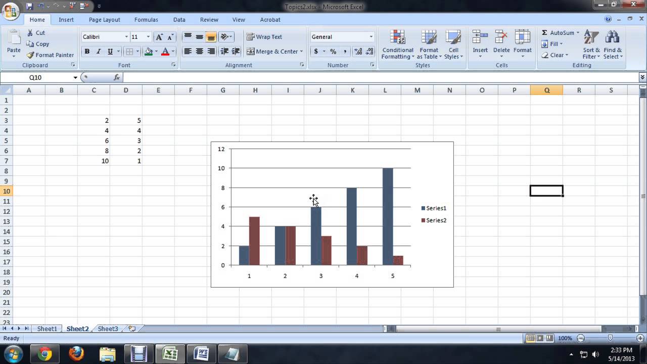
A bar graph helps you display data using rectangular bars, where the length of each bar is a numeric value depending on the category it belongs to. Let’s move on to understand how to create a bar graph in an easy and simple way. Bar graphs are mainly used to make comparisons across a range. If you want to display the animals (instead of the months) on the horizontal axis, execute the following steps. Excel also has a Recommended Charts feature that can suggest the right chart type for your data. To create a chart in Excel based on a specific chart template, open the Insert Chart dialog by clicking the Dialog Box Launcher in the Charts group on the ribbon.

Simply select the existing chart, switch to the Insert tab and choose another chart type in the Charts group. To make your Excel graph easier to understand, you can add data labels to display details about the data series. Depending on where you want to focus your users' attention, you can add labels to one data series, all the series, or individual data points. Creating graphs in Excel is like turning your data into a story. With just a few clicks, you can take rows and columns of numbers and turn them into a visual masterpiece.
For example, you can combine a column or area chart with a line chart to present dissimilar data, for instance an overall revenue and the number of items sold. When the chart options pop up — either on the ribbon or under your cursor if you right-clicked — you’ll next click Change Chart Type. A menu will pop up with a variety of chart type options on the left.

After you input your data and select the cell range, you’re ready to choose the chart type. In this example, we’ll create a clustered column chart from the data we used in the previous section. For more chart types, click the More Column Charts… link at the bottom.
Reorder your data, if desired.
And you won’t be left wondering about who has the latest data sets. Most project management solutions, like Workzone, have file sharing and some visualization capabilities built-in. To change colors or to change the design of your graph, go to Chart Tools in the Excel header. You will see it transform into a tiny arrow pointing downwards. When this happens, click on the cell A and the entire column will be selected.
Pingboard Organizational Chart Template
If you have imported this data from a different software, then it’s probably been compiled in a .csv (comma separated values) formatted document. Graphs represent variations in values of data points over a given duration of time. They are simpler than charts because you are dealing with different data parameters. Comparing and contrasting segments of the same set against one another is more difficult. A pie chart is a circular graph that represents data by dividing the circle into sectors, where each sector illustrates a proportion to the whole. A pie chart is nothing but a circular graph representing data in the form of a pie/circle.
Graphs allow you to roughly compare data within a set, not dig into it. No one's looking at your graph to see incremental differences between data points -- they want to see general, overarching trends. To order the graphs in Excel, you'll need to sort the data from largest to smallest. Click 'Data,' choose 'Sort,' and select how you'd like to sort everything.
How to Create a Panel Chart in Excel - MUO - MakeUseOf
How to Create a Panel Chart in Excel.
Posted: Fri, 17 Mar 2023 07:00:00 GMT [source]
Let's start by introducing our Excel worksheet so you understand what we aim to achieve with this blog. Alternatively, you can right-click anywhere within the graph and select Change Chart Type… from the context menu. Click the arrow next to Axis, and then click More options… This will bring up the Format Axis pane. Or, you can click the Chart Elements button in the upper-right corner of the graph, and put a tick in the Chart Title checkbox. His writing has appeared on dozens of different websites and been read over 50 million times. The first thing you need to do is select the data you want to include in your graph.
By paying attention to the aesthetic details of your dashboard, you’ll create a tool that not only provides valuable insights but also encourages user adoption and engagement. It’s easy to create charts and graphs in Excel, especially since you can also store your data directly in an Excel Workbook, rather than importing data from another program. Excel also has a variety of preset chart and graph types so you can select one that best represents the data relationship(s) you want to highlight. By following the steps outlined in this tutorial, you can easily create professional-looking graphs for your presentations, reports, and analyses. For specific chart types, such as pie chart, you can also choose the labels location.
Then, go to the Insert tab and click the column icon in the charts section. Microsoft Excel is an incredibly powerful tool for managing and analyzing data. However, creating visually appealing charts from raw data can be a challenging and time-consuming process. Microsoft Excel determines the most appropriate gridlines type for your chart type automatically. For example, on a bar chart, major vertical gridlines will be added, whereas selecting the Gridlines option on a column chart will add major horizontal gridlines. For most chart types, the vertical axis (aka value or Y axis) and horizontal axis (aka category or X axis) are added automatically when you make a chart in Excel.
The collection ranges from basic charts like bar, line, and pie charts to more innovative designs. To format the axis title, right-click it and select Format Axis Title from the context menu. The Format Axis Title pane will appear with lots of formatting options to choose from. You can also try different formatting options on the Format tab on the ribbon, as demonstrated in Formatting the chart title. To make a bar graph, highlight the data and include the titles of the X- and Y-axis.
Another popular chart is a waterfall chart, which is essentially a series of column graphs that show positive and negative changes over time. There is no Excel preset for a waterfall chart, but you can download a template to help make the process easier. For a full walkthrough, read How to Create a Waterfall Chart in Excel. Organizations of all sizes and across all industries use Excel to store data. While spreadsheets are crucial for data management, they are often cumbersome and don’t provide team members with an easy-to-read view into data trends and relationships. Excel can help to transform your spreadsheet data into charts and graphs to create an intuitive overview of your data and make smart business decisions.


No comments:
Post a Comment